iNMR | Advanced J Management

The J Manager as a Center of Gravity

There is a little module that helps you to:

Store chemical shifts and coupling constants.
Calculate them from the output of peak-picking or other internal sources.
Report the values either as text or as graphic.

It's called the J Manager. What it can't do is to check the consistency of your data. What it's not supposed to do is to take strategic decisions. It can't choose the best method among the many ones available (peak-picking, line-fitting, quantum-mechanical simulation, 2D-NMR...). Don't forget that the simplest and fastest method is not always the most accurate one. This tutorial compares a few of the afore-mentioned methods and provides you with a training field. The purpose is merely to show what's available into the program, not to evaluate the pros and cons of each alternative.

In recent years other commercial software programs have introduced “first-order-multiplet-analyzers” and marketed them as the solution to extract the NMR parameters. That is a limited view, because not all multiplets are first-order and, even when they are, they can be hidden or unresolved. The J Manager included into iNMR is an open tool that can organize information coming from the rest of the program or even from outside. It works like a hub: accepts many kinds of input and offers several outlets.

For full understanding, the reader should be an expert iNMR user who has already browsed both the J Manager Primer and the Line Fitting Primer. The simplest usage of the J Manager consists in manually typing the spectroscopic parameters directly into the table. It's what you do when you have measured the J in a 2D experiment and want to store it into the table of the 1D counterpart. Another example is when you measure a coupling constants reliably in a multiplet and want to copy the same value into the row of the coupling partner, whose multiplet is hidden for some reason. This kind of 100% manual usage needs no explanation.

To follow the present tutorial in practice, download this (compressed) folder. It contains an imaginary A₂B₂CD spectrum in two formats:

A simulation document (“A2B2CD.spins”) in which you can modify the single parameters. It's included for documentation, but we're not gonna use it.
The same plot with some authentic noise (taken from a true NMR spectrum) added. This will be our training field.

It would be a big surprise to find a chemical compound with a spectrum like this. Should we care? This artificial spectrum has nothing to demonstrate. The only purpose is to let the reader familiarize with the commands and controls of iNMR.

Peak Picking

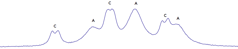
The A signal (a triplet) and the C signal (a triplet of doublets) both fall at 3 ppm.

Let's start, alphabetically, from A. Peak-pick the 3 lines below (use the peak-picker tool to click each of the lines). Then select the gray region with the mouse.

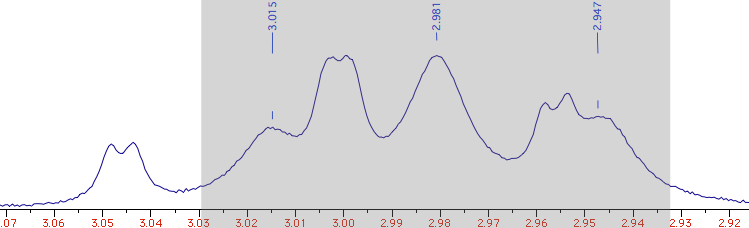
Open the J Manager and click the first icon (“extract”). It will extract a triplet (J = 6.75 Hz). It's called “A” simply because whatever fills the first row in the table gets that name, initially (in our case, it's a matter of coincidence). Change the number of Hs from 1 to 2.
Delete the peak-picking labels and create 6 new ones:

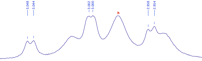
Select them all; press the key “e” (a shortcut for “extract”); A new row appears into the table. The Js, this time, are 9.00 and 0.73 Hz. Note how the peak has been called “B”. You can correct it manually, if desired. The multiplets of the true B and D can be analyzed in the same way.

Line Fitting

Select the region between 2.935 and 3.055 ppm. Issue the command “Simulate/Deconvolution”. A new module appears. Click the icon “smooth” 3 times (wait an instant each time to see what happens). You should get this list of 7 peaks:

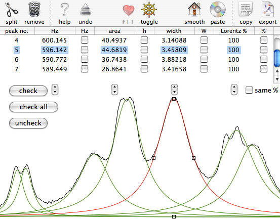
Select the line no. 6 and click the icon “split”. Do the same with the line no. 4. Resize and relocate the new lines:

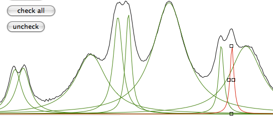
Click the buttons “check all”, then “same %”, then “FIT”. Click the latter as many times as you like, then click “copy”. This is the text you have copied into the clipboard:

Parameters for 9 peaks
  frequency (Hz)     intensity      width (Hz)   Lorentzian %

       609.7107         4.1123         1.0006       100.0000
       608.7083         4.3374         1.0259       100.0000
       603.1718        15.8642         2.8998       100.0000
       600.6833        10.5970         1.3038       100.0000
       599.7023         9.4219         1.2068       100.0000
       596.1126        36.1430         2.9834       100.0000
       591.7272         4.8997         1.0157       100.0000
       590.7509         4.9139         1.0377       100.0000
       589.1394        20.2227         3.0599       100.0000

Save it somewhere, because we'll need it soon. Let's call it the “list of 9 peaks”. Now return to the deconvolution window and delete the 6 lines corresponding to multiplet C. Press “copy”. Open the J Manager for the main spectrum and click “paste”. It calculates a triplet whose J = 7.02 Hz. Note how, this time, the number of Hs is correctly estimated.
Copy the “list of 9 peaks” into the clipboard. Return to the deconvolution window and paste it. This action restores the table. Remove the 3 lines belonging to A. Click “copy”. Reach the J manager and click “paste”. The new calculated Js are 0.99 and 8.99 Hz.
A similar, yet simpler, process can be applied to the isolated multiplets B and D.

Quantum Mechanics

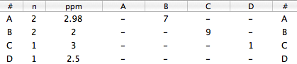
Press Cmd-N. A table with two rows is created. Click the button “add row” twice. There are 4 rows now. Fill the values:

Close the dialog. Possibly change the color for this simulated spectrum (We'll use the red for our picture). Open the Overlay Manager (Cmd-Shift-O) and select the other spectrum. Close the Overlay Manager. Click the icon “assimilate” (to match the Larmor frequencies of the two spectra).

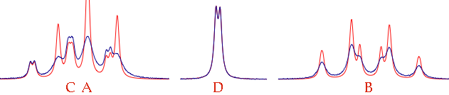
Check the parameter “defW” into the drawer. Issue the command: “Simulate/Fit to Overlay”. The two spectra will be more similar after the iteration, but not enough. Reopen the table (command: “Simulate/Define Systems...”). Uncheck the option: “same width for all lines”. Close the table. Now check WA, WB and WC and start a new iteration (“Fit to Overlay”). If the fit improves, go the extra mile. Check all the parameters, from “pop” down to the bottom. Start the definitive iteration.

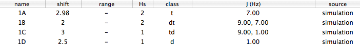
When the fit is perfect, all we have to do is to move the information from one window to another. Issue the command “Simulate/Listing...”. Select the text that appears:


nucleus n   shift      multiplicity    Js

1A      2   2.9800              t     7.00
1B      2   2.0000             dt     9.00, 7.00
1C      1   3.0000             td     9.00, 1.00
1D      1   2.5000              d     1.00

The decimal digits are mostly zeroes, just because the “experimental” spectrum has been created on my computer... Go to the J Manager and paste. This time, the names too are imported: